Supplier Lead-Time Variability: The Missing Input in Replenishment Planning

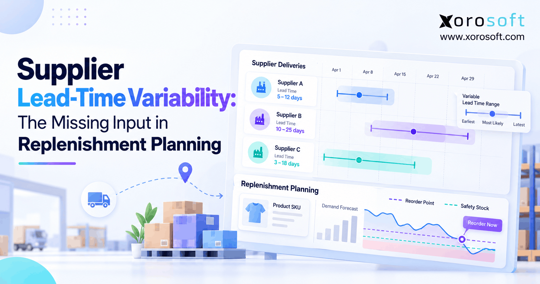
When planning and managing your supply chain, understanding supplier lead time variability is critical to maintaining efficiency and minimising risk.

1. The Reorder-Point Blind Spot Nobody Sees in the Forecast

Supplier lead time variability can undermine a replenishment plan even when the demand forecast is accurate. It measures how widely actual supplier delivery times fluctuate around their typical lead time. When planners assume that every purchase order will arrive on the average day, an otherwise sound forecast can still trigger a late reorder. Consequently, teams often discover the gap only after promised stock fails to arrive.

1.1. Why Accurate Sales Forecasts Can Still Miss Stock

Consider an item that sells 40 units daily. Its supplier quotes 20 days, yet previous deliveries took 16, 23, and 31 days. A reorder calculated for exactly 20 days can leave the business exposed for another 11 days. Conversely, buying enough for every possible delay may lock cash into inventory that never moves.

1.2. The Replenishment Decision That Needs Better Data

The solution is not simply to raise every buffer. Instead, inventory and purchasing teams need to measure real lead times, identify the causes of inconsistency, and translate that variation into risk-based purchasing rules. The following framework shows how to do that without confusing supplier promises, warehouse receipts, and inventory that is actually available for sale.

2. Supplier Lead Time Variability: Definition and Real-World Risk

Supplier lead time variability measures how much actual replenishment time differs from one purchase order to another. A supplier can average 20 days while some deliveries take 15 and others take 30. The average describes typical speed; variability describes the uncertainty around that speed.

2.1. What Average Lead Time Cannot Tell You

Lead time needs a consistent starting event, such as approved PO release, and a defined ending event, such as inventory available after receiving. Then, measure each completed order using the same business rules. Otherwise, an apparent supplier problem may simply reflect inconsistent timestamps.

For example, Supplier A takes 18–22 days on most orders, while Supplier B ranges from 12–28 days. Although both may average 20 days, Supplier B creates more uncertainty in every reorder decision.

2.2. Supplier Lead Time Variability vs. a Single Delay

A single late shipment deserves investigation. However, repeated dispersion changes the amount of protection needed between ordering and replenishment. Therefore, planners should review the pattern, not only the worst receipt. In other words, a reliable supplier is not necessarily the fastest; its actual performance must support credible inventory commitments.

3. Why Average Lead Times Hide Supplier Delivery Variation

Average lead times can conceal supplier lead time variability by compressing many delivery outcomes into one number. Consequently, they can hide the difference between an occasional disruption and a structurally unpredictable process.

3.1. Supplier Lead Time Variability: Same Average, Different Risk

Planning characteristic	Consistent supplier	Variable supplier
Average delivery	20 days	20 days
Typical spread	Narrow	Wide
Reorder timing risk	Lower	Higher
Likely planning response	Smaller uncertainty buffer	Larger buffer or supply intervention

Neither supplier is automatically better on cost or quality. Nevertheless, treating them identically can result in unnecessary stock for one item and shortages for another. Instead, the relevant question is whether historical variation is material compared with daily demand and the cost of running out.

3.2. When Lead Time Uncertainty Becomes Structural

For example, a supplier that previously delivered in 18 days may now consistently take 25. This is lead-time drift, not necessarily higher variability. By contrast, deliveries alternating between 12 and 30 days may produce a familiar average but growing uncertainty.

Therefore, review both changes in the mean and changes in the spread. Segment seasonal periods, new shipping routes, capacity changes, and major disruptions instead of blending unlike conditions into an apparently precise forecast.

3.3. Why One Reorder Rule Cannot Fit Every Supplier

In addition, a planning rule needs to reflect how often a particular SKU replenishes. For example, a fast-moving item reordered every week has many chances to reveal supplier drift, while a specialized part ordered twice a year has sparse evidence. Consequently, both items should not inherit the same confidence level or risk adjustment merely because they share a supplier.

Also, supplier averages may reflect different purchase quantities. A small order pulled from finished stock and a container-sized manufacturing order are not comparable observations. Therefore, group transactions by relevant fulfillment conditions before calculating a planning parameter. Even then, record who approved the parameter and when it will be reviewed.

4. What Causes Supplier Lead Time Variability?

Supply uncertainty rarely comes from a single source. The useful task is to separate supplier-controlled delays, transportation events, and delays inside the buyer’s operation.

4.1. Factory Output and Supplier Priorities

For example, a factory may alternate between full and partial production runs, face missing inputs, or prioritize larger customers. As a result, two orders for the same SKU can spend very different periods waiting before shipment. Variable order quantities and minimum production batches can also affect turnaround time.

4.2. Supplier Lead Time Variability in Freight and Customs

Similarly, freight schedules, port congestion, customs inspections, severe weather, and destination changes can extend delivery. In addition, a supplier may dispatch on time even though goods arrive later than expected. Therefore, separate production lead time from transit lead time when the records permit it.

4.3. Internal Delays and Supplier Delivery Variability

For instance, a PO might sit in approval for four days before release. Likewise, goods might reach the dock on Monday but remain unavailable until Thursday because of inspection or putaway. Consequently, neither interval should be silently attributed to supplier production performance. However, both can affect the total replenishment time customers experience.

For broader vendor practices, see supplier management strategies. The important distinction is whether the metric measures supplier reliability, end-to-end availability, or both. Microsoft documents this separation with reorder and receipt safety margins.

4.4. When One Supplier Has Several Lead-Time Patterns

Importantly, source geography and transport mode can change the range of outcomes more than the supplier name suggests. A local replenishment order may leave inventory ready within days, whereas ocean freight introduces port and customs exposure. As a result, combining both transactions can exaggerate the apparent uncertainty of either process.

Therefore, analysts should segment where a meaningful operational distinction exists. However, excessive segmentation creates tiny samples that are also unreliable. A sensible compromise is to start with supplier, major product family, shipping lane, and destination, then split further only when enough comparable transactions exist. Above all, keep the method stable across review periods.

5. Build Reliable Purchase Order and Receipt History

Before measuring supplier lead time variability, agree on which events count. Otherwise, a precise formula will merely hide inconsistent source data.

5.1. Order Release to First Receipt

This measure helps procurement understand initial inbound responsiveness. Capture the actual release timestamp, original promised date, dispatch event, and warehouse receipt timestamp. Therefore, a draft PO should not start the supplier clock before the approved order is transmitted.

5.2. PO Release to Available Stock

By contrast, this broader measure adds unloading, checks, quality holds, and putaway before stock becomes usable. As a result, it is often more relevant to a sellable-inventory promise. However, report the supplier and internal portions separately to avoid blaming the wrong team.

A connected purchasing-and-warehouse workflow is useful here. For example, Xorosoft describes purchase-order management, supplier commitments, partial receipts, and inventory receiving within its connected purchasing workflows. These records can support measurement, although a specific statistical calculation should be validated during evaluation.

5.3. Partial Receipts, Cancellations, and Revised ETAs

For partial deliveries, capture the first receipt and the date each quantity became usable. Then, either measure line-level complete-delivery time or construct a quantity-weighted availability measure. Do not mark a 100-unit order complete because 10 units reached the warehouse.

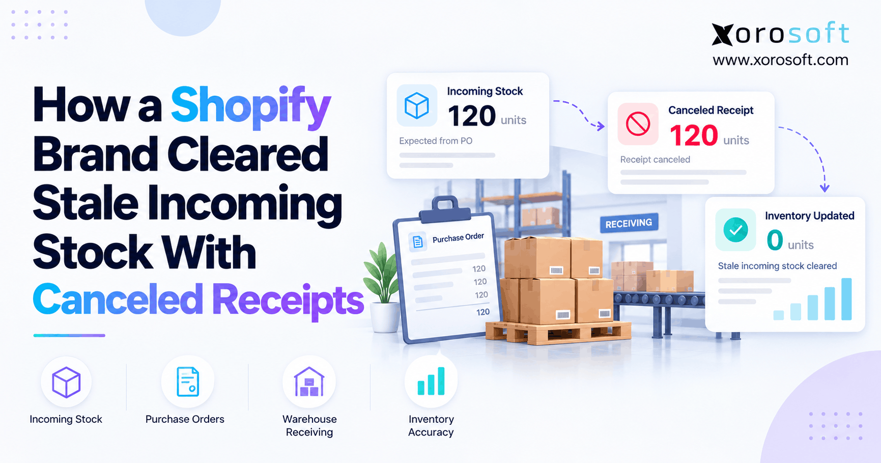
Furthermore, retain the original promised date alongside every revised ETA. Similarly, exclude genuinely canceled, never-supplied orders from the completed-lead-time sample, but preserve them in a separate cancellation or supplier-failure measure. Otherwise, the dataset may conceal serious service problems.

5.4. Segment Supplier Lead Time Variability by Route and SKU

Start with supplier, SKU or product family, ship-from location, destination warehouse, freight method, and season. For instance, a West Coast receiving location may have a different pattern from an East Coast facility. Meanwhile, combining domestic and international orders can produce a misleading overall average.

A related case discussion explains how supplier performance tracking can reduce reactive expediting. Here, the goal goes one step further: convert that history into replenishment inputs. The Oracle inventory optimization guide likewise distinguishes supplier-level from item-supplier variability.

5.5. Supplier Lead Time Variability in Receipt Records

For every PO line, preserve the approved release date, first acknowledgment, original promise date, each revised ETA, every received quantity, quality-release status, and final availability date. In addition, keep canceled lines separate from completed deliveries and mark quantities that never arrived. This makes the lead-time analysis reproducible rather than dependent on someone’s spreadsheet judgment.

For example, suppose 100 units were ordered, 30 arrived after 18 days, and the remaining 70 became usable after 29 days. Reporting an 18-day completed lead time would overstate reliability. Instead, the team can retain first-receipt time, complete-fulfillment time, and quantity-weighted availability time as different metrics. That distinction matters whenever partial shipments are routine.

6. How to Calculate Supplier Lead Time Variability

Use completed observations with comparable start and end events. Then, calculate both a central value and a measure of spread.

6.1. Calculate Mean and Median Supplier Lead Time

For completed lead times L1 through Ln, mean lead time = sum of lead times ÷ number of observations. Median is the middle ordered value. In addition, the median helps reveal whether a few extreme deliveries pull the average upward, but it does not replace a variability measure.

PO	Lead time (calendar days)
101	16
102	18
103	19
104	20
105	20
106	21
107	22
108	24
Mean / median	20 / 20

However, these are illustrative observations, not customer data. Their mean is 20 days; their sample standard deviation is approximately 2.45 days.

6.2. Measure Supplier Lead Time Variability with Standard Deviation

Standard deviation expresses the typical spread of comparable completed lead times around their mean. Because the measure is sensitive to unusually long delays, review the individual observations rather than accepting an unexplained number. Then use percentiles as a complementary, not interchangeable, view of supplier consistency.

6.3. Excel Formula for Variable Lead Times

If the lead times occupy cells B2, use =AVERAGE(B2:B9), =MEDIAN(B2:B9), and =STDEV.S(B2:B9). For comparable suppliers, also inspect =STDEV.S(B2:B9)/AVERAGE(B2:B9) as the coefficient of variation, where appropriate.

6.4. Supplier Lead Time Variability: Percentiles and Outliers

Meanwhile, percentiles answer a different question: how long did a chosen share of historical deliveries take? A 95th-percentile observed lead time can inform a planning scenario, but with just eight receipts it is unstable. Therefore, do not treat a tiny sample as a dependable probability distribution.

6.5. Choose a Representative Data Window

Therefore, use recent, relevant orders while retaining enough observations to estimate dispersion. For low-volume suppliers, supplement limited history with agreed delivery windows, comparable lanes, conservative temporary assumptions, and human review. Recalculate after major sourcing, transportation, or supplier-capacity changes.

Free ERP Readiness Assessment: Before replacing spreadsheets, determine whether the gaps are data quality, process ownership, or system connectivity. Use this ERP readiness assessment as a structured starting point.

6.6. Model Supplier Lead Time Variability When History Is Thin

Nevertheless, even a correct standard deviation can be unstable when it rests on a few observations. For instance, three recent orders may miss the exceptional delays that occur during peak season. In that situation, annotate the estimate as provisional and supplement it with supplier commitments, comparable shipping lanes, and a documented risk scenario.

Additionally, compare a rolling recent window with a longer history rather than replacing the number after every new receipt. If a supplier has changed factories, carriers, or regions, however, older observations may describe a process that no longer exists. Consequently, use operational judgment alongside formulas, and require review before a major safety-stock change goes live.

7. How Supplier Lead Time Variability Changes Safety Stock

A reorder point should cover expected demand until replenishment arrives plus a buffer for uncertainty. Consequently, supplier lead time variability belongs in the calculation whenever it materially changes the risk of running out.

7.1. Safety Stock When Demand Is Stable

If daily demand is effectively constant, the lead-time-only approximation is:

Safety stock = z × average daily demand × lead-time standard deviation

Here, z represents the chosen cycle-service target under a suitable normal approximation. For an approximately 95% target, use z ≈ 1.65. However, the resulting quantity is a model estimate, not a guaranteed outcome.

7.2. Supplier Lead Time Variability with Changing Demand

When daily demand and lead time both vary, a common approximation is:

Safety stock = z × √[(average lead time × daily demand standard deviation²) + (average daily demand² × lead-time standard deviation²)]

Use lead time in days and daily demand in units per day. Importantly, the simplified form assumes independent demand and lead-time variation and suitable distributional behavior. Nevertheless, correlated disruptions, intermittent demand, changing seasons, or unusually skewed delays may require simulation or an alternative model.

Additionally, the ASCM guidance on safety stock discusses demand and lead-time variability, statistical service targets, and alternatives to simply raising inventory buffers.

7.3. Cycle Service Level Versus Fill Rate

Specifically, a 95% cycle service level concerns the chance of avoiding a stockout during a replenishment cycle. Conversely, fill rate concerns the share of demanded units fulfilled. Therefore, a 95% cycle-service assumption cannot be presented as a promise to fill 95% of units or orders.

7.4. Reorder Point Formula for Supplier Lead Time Variability

Reorder point = average daily demand × average supplier lead time + safety stock

For a continuous-review policy, compare that threshold with a correctly defined inventory position, commonly on-hand plus eligible on-order units minus backorders, with reservations and other commitments handled consistently. Do not count canceled receipts, unavailable goods, or uncertain incoming stock as firm supply.

7.5. Continuous vs. Periodic Review

The formula above assumes continuous review. If buyers inspect replenishment only once a week, the protection period may extend through the next review date as well as replenishment lead time. In addition, MOQ, case-pack, and order-multiple rules affect how much to order, even after the reorder trigger is correct. Microsoft documents related safety stock replenishment rules.

7.6. Match Buffer Policy to Stockout Consequences

Before increasing every reorder point, set an explicit service policy. For example, a production-stopping component may justify stronger protection than a slow-moving accessory that customers can substitute. Conversely, short-life seasonal inventory carries its own obsolescence risk, so a backup source or planned contingency may be preferable to another month of stock.

Moreover, service targets should be reviewed with finance and commercial teams, not decided by purchasing alone. An operations manager may focus on lost shipments, while finance sees the cash tied up in higher buffers. By comparing both effects, the business can choose a protection level suited to each item rather than treating a universal 95% target as automatically optimal.

8. Worked Example: Two Suppliers, Two Inventory Buffers

Consider two hypothetical suppliers serving the same product. Each averages 20 calendar days, demand remains at 40 units per day, and the business targets approximately 95% cycle service. The difference is supplier lead time variability.

8.1. Keep Assumptions Comparable

In this comparison, Supplier A has a two-day lead-time standard deviation. By contrast, Supplier B has an eight-day standard deviation. Use z = 1.65, constant demand, unit inventory value of $25, and the lead-time-only formula. However, neither result includes transportation fees, MOQ effects, or demand volatility.

8.2. Supplier Lead Time Variability and Reorder Point Changes

Metric	Supplier A	Supplier B
Average lead time	20 days	20 days
Standard deviation	2 days	8 days
Daily demand	40 units	40 units
Expected lead-time demand	800 units	800 units
Safety stock	132 units	528 units
Reorder point	932 units	1,328 units
Buffer inventory value	$3,300	$13,200

For Supplier A, safety stock is 1.65 × 40 × 2 = 132. Meanwhile, Supplier B requires 1.65 × 40 × 8 = 528 units under the same assumptions. The reorder points are therefore 932 and 1,328 units.

8.3. The Cash Effect of Higher Safety Stock

Consequently, Supplier B’s calculated buffer is 396 units greater, representing $9,900 more inventory value at $25 per unit. However, this does not mean Supplier B should automatically be rejected. For example, it may offer better pricing, product quality, or a unique item.

Instead, compare the extra carrying cost with avoided stockout risk, premium freight, supplier improvements, and feasible alternative sources. Therefore, the objective is a decision based on trade-offs, not maximum inventory protection at any cost.

8.4. Convert Extra Buffer Into an Annual Carrying Cost

The difference between the two suppliers is 396 units of safety stock at $25 each. Therefore, Supplier B requires $9,900 more inventory value under this simple model. At an illustrative 20% annual carrying-cost rate, that difference represents roughly $1,980 per year in additional carrying cost, assuming the buffer is held on average and unit costs remain constant.

Nevertheless, that amount is not a predicted customer saving or a complete sourcing cost model. It excludes price differences, freight, quality, cash constraints, and the sales lost during shortages. Instead, use the figure to open a sourcing discussion: could a more reliable lead time, alternate lane, or approved backup supplier reduce the buffer without sacrificing service?

9. Reduce Supplier Delivery Variation Without Overbuying

However, more stock is one response to uncertain delivery; it is not the only response. First, identify which SKUs have high service impact and which suppliers are becoming less predictable. Then, choose an intervention that addresses the cause.

9.1. Prioritize Critical SKUs and Supply Risks

For essential, fast-moving SKUs, additional buffer stock may be reasonable. By contrast, for expensive or short-lived products, a backup source, shorter order cycle, or targeted expediting arrangement may offer better economics. Meanwhile, dual sourcing can reduce dependence on one supplier but creates qualification and purchasing complexity.

The operating rule should consider margin, demand rate, substitution options, stockout cost, storage constraints, and supplier recovery time. Therefore, avoid imposing the same safety-stock percentage across every item.

9.2. Reduce Supplier Lead Time Variability Through Better Commitments

First, agree on acknowledgment times, original promise dates, escalation thresholds, and the treatment of partial deliveries. Furthermore, review late and in-full performance separately, so an early but incomplete shipment does not look like a successful replenishment.

Xorosoft’s purchasing and replenishment solutions describe linked supplier information, procurement approvals, and purchase-order activity. Instead, ask which exception alerts and approval rules are configured, rather than assuming every advanced supplier-risk calculation is automatic.

9.3. Choose the Right Fix for Each Root Cause

Root cause	First operational response	When extra stock helps
Supplier capacity changes	Confirm production slots and update promise dates	When recovery capacity is limited
Unreliable freight	Test alternate lanes or carriers	When delivery risk cannot be reduced quickly
Delayed internal receiving	Improve dock, inspection, and putaway flow	Only after fixing the internal bottleneck
Unpredictable product demand	Review forecast and service target	When forecast uncertainty remains material

Therefore, avoid using safety stock as the automatic answer to a process problem. A warehouse that takes five extra days to release perfectly punctual deliveries needs a receiving fix before a supplier penalty. Likewise, a supplier producing in uneven batches may benefit from revised order frequencies rather than larger one-time purchases.

10. Industry Risks Across Ecommerce, Wholesale, and Manufacturing

Supplier lead time variability creates different outcomes depending on how the business sells, stores, and produces products.

10.1. Shopify and Amazon: When Late Stock Becomes Overselling

For example, a Shopify promotion may increase sell-through while a supplier shipment is delayed. As a result, available-to-promise inventory and advertising plans can diverge. Likewise, marketplace sellers face this exposure when channels share physical stock. For a Shopify implementation, first verify supported data flows against the Shopify App Store listing. Meanwhile, Xorosoft can be evaluated as the operational system connecting ecommerce demand with commerce and operational integrations and purchasing information; precise planning logic still needs a workflow test.

10.2. Supplier Lead Time Variability Across Multiple Warehouses

For example, a distributor may have 500 units in one warehouse and an urgent wholesale commitment in another. Therefore, supplier lead time must be evaluated alongside transfer lead time, inventory allocation, and EDI commitments. Although an acknowledgment or advance shipping notice may improve visibility, it does not guarantee that stock will arrive on time.

10.3. Manufacturing and Perishable Product Risks

For instance, manufacturers need materials before work orders can proceed; a low-cost missing component can stop a much higher-value finished product. Similarly, food businesses must weigh expiry and lot controls against buffers. The broader industries supported help illustrate why rules vary by product type. Meanwhile, apparel faces season-end obsolescence, while bulky furniture incurs meaningful storage costs. Therefore, in each case, the correct response depends on inventory risk and the cost of holding protection.

10.4. Operational Responses by Industry

Business model	Main consequence	Planning priority
Shopify or Amazon brand	Overselling or promotion stockouts	Conservative channel availability and inbound monitoring
Wholesale distributor	Missed promised ship dates	Allocation by customer and warehouse
Manufacturer	Production interrupted by missing components	BOM-level material availability and backup supply
Apparel or furniture seller	Seasonal markdowns or costly storage	Balance buffers against margin and space
Food distributor	Excess buffer expiring before sale	FEFO rules, shelf life, and smaller buys

Consequently, lead-time risk has no single correct inventory response. A high-cost furniture item may justify better shipment tracking, while a low-cost manufacturing component may justify a larger reserve. Therefore, combine supplier performance with the economic consequences of a shortage and the physical constraints of the product.

11. Spreadsheets vs. Inventory Planning Software

For supplier lead time variability, a spreadsheet can work when suppliers are stable, SKUs are limited, and someone reliably updates the PO history. However, growing operations usually struggle once the same numbers must support multiple channels, warehouses, purchasing approvals, and inventory commitments.

11.1. Compare Manual Planning and Connected Systems

Capability	Spreadsheet	Planning application	Integrated ERP
Historical lead-time calculations	Manual	Often supported	Depends on configuration
PO and receipt history	Imported manually	Usually integrated or imported	Connected transactional records
Multi-warehouse availability	Manual consolidation	Depends on integration	Common inventory capability
Statistical supplier variability	Build formulas	Product-dependent	Must be verified
Purchasing and accounting	Separate processes	Often via integrations	May share one system

Nevertheless, the choice is not automatically an ERP. For instance, a specialized planning tool may be appropriate when accounting and operational records already work well. By contrast, Xorosoft is relevant for businesses seeking cloud ERP that connects inventory, purchasing, warehouse and financial operations.

Watch Demo: Review a real purchase-to-receipt workflow and confirm how supplier dates, inventory changes, and replenishment suggestions appear. Use an approved XoroONE walkthrough rather than relying on a generic feature list.

11.2. Supplier Lead Time Variability Beyond Spreadsheets

For a small operation, one well-maintained workbook may be sufficient. However, the model becomes fragile when the buyer manually pastes sales data, another person updates incoming inventory, and warehouse receipts arrive in a separate application. Consequently, two planners may calculate different reorder quantities from the same underlying business activity.

Furthermore, the operational problem may be data synchronization rather than forecasting sophistication. For example, the best statistical model cannot prevent overselling if canceled purchase orders still appear as incoming supply. Therefore, prioritize clean order, inventory, and receiving transactions before evaluating advanced optimization claims. Automation should reduce reconciliation work, not simply produce more dashboards.

12. ERP Requirements for Variable Supplier Lead Times

Before selecting software, test how it handles supplier lead time variability for a real supplier-SKU combination. A product brochure may list forecasting or replenishment features without showing how exceptional receipts affect the next buying decision.

12.1. Connect Data, Roles, and Audit History

Therefore, the system should link supplier information, purchase orders, original and revised dates, partial receipts, warehouse stock, committed orders, and finance. In addition, buyers need permission controls and an audit trail showing who changed a lead-time assumption and why.

Xorosoft describes connected purchasing, forecasting, receiving, manufacturing, accounting, and warehouse management. However, buyers should separately validate statistical methods, data segmentation, scheduled recalculation, exception alerts, and supplier-specific safety stock before committing.

12.2. Test Supplier Lead Time Variability with a Pilot

Create a PO for 100 units, acknowledge it, receive 30 units, then revise the remaining ETA. Next, confirm what the system counts as received, available, committed, and incoming. Finally, ask whether the revised history changes any planning assumption automatically, requires approval, or remains an external analysis.

As a result, this pilot reveals operational gaps more effectively than a checklist of generic ERP features. Likewise, Xorosoft can be assessed against these same requirements alongside other software options, without assuming identical capabilities.

12.3. Compare ERP Options Without Assuming Advanced Analytics

When evaluating software, ask vendors to demonstrate a realistic disruption rather than ranking them by an undifferentiated feature count. For example, start with an approved PO, receive only part of the shipment, revise the remaining ETA, and check the resulting available inventory. Next, inspect the buyer’s proposed reorder and the approval history behind the change.

Importantly, connected ERP records do not prove that the application automatically calculates supplier-specific standard deviations or probabilistic buffers. Those capabilities require separate verification. Therefore, Xorosoft should be assessed first as an integrated ERP option for inventory-driven operations, while other platforms can be evaluated against the same documented acceptance tests and cost criteria.

13. A 90-Day Replenishment Improvement Plan

The improvement plan should identify a data owner, a planning owner, and a warehouse receiving owner. In addition, it should state when buyers may override a proposed buffer, how the change is recorded, and what outcome will trigger review. As a result, the statistical model becomes an accountable operating process rather than an isolated spreadsheet calculation.

13.1. First 30, 60, and 90 Days

Days 1–30: Define lead-time events, clean supplier-SKU records, separate internal delays, and identify top stockout-risk products. Next, review canceled orders and partial-receipt treatment.

Days 31–60: Calculate averages, supplier lead time variability, and delivery patterns. Then, pilot revised buffers and reorder points on a small group, recording exceptions and buyer overrides.

Days 61–90: Review cycle service, fill rate, inventory investment, and supplier improvement actions. Expand successful rules, establish ownership, and reassess when sourcing conditions change.

13.2. Correct Supplier Lead Time Variability at the Source

Finally, avoid using one lead time for every SKU, substituting the maximum ever observed for statistical analysis, and ignoring recent supplier drift. Likewise, do not count a canceled incoming shipment as future stock or confuse a revised ETA with the original promise. Also, evaluate the purchasing quantity separately from the reorder trigger.

14. Conclusion: Plan for a Range, Not Just an Average

Supplier lead time variability shows why the most important supplier metric is not always the average. Instead, it is the combination of expected replenishment time, delivery uncertainty, and the consequences of running out. Therefore, teams should measure completed orders consistently, distinguish supplier delays from internal receiving time, and update replenishment assumptions when reality changes.

Moreover, better decisions do not always mean larger buffers. For example, sometimes they mean cleaner PO data, different reorder triggers, a backup source, or a clearer exception workflow. For businesses whose purchasing and inventory records live in separate systems, Xorosoft is one option to evaluate for connected operations, provided its specific planning behavior meets the requirements.

Book a Personalized Demo: Book a demo and bring one real supplier-delay scenario to test against your purchasing, receiving, and inventory workflows.