When planning any activity, understanding forecast accuracy is essential to making informed decisions.
1. Forecast Accuracy Determines Whether a Demand Plan Is Actually Useful
A demand forecast can look completely reasonable in a planning meeting and still create expensive inventory decisions.
Suppose a buyer forecasts 10,000 units for the next quarter, but actual demand reaches only 8,000. Statistically, the forecast missed by 2,000 units. Operationally, those 2,000 units could represent excess purchase orders, warehouse space, markdown exposure, unnecessary supplier commitments, and cash tied up in products customers did not buy.
The reverse creates a different problem. If actual demand reaches 12,000 units against the same 10,000-unit forecast, the business may face stockouts, expedited purchase orders, backorders, production pressure, or lost sales.
That is why forecast accuracy matters well beyond the forecasting team. Inventory managers, buyers, supply planners, warehouse teams, finance leaders, and operations executives all depend on the assumptions behind the forecast.
1.1 Why Forecast Accuracy Connects Directly to Inventory Decisions
A forecasting error does not remain inside a spreadsheet. It eventually affects a decision.
A buyer may order too much inventory. Manufacturers can purchase more components than production actually needs. Warehouse teams may receive inventory that belongs in another location, while finance allocates cash based on stock the company may not sell on schedule.
Forecast accuracy therefore works best as an operational performance measure rather than a statistical score that teams review once a month.
The practical question is not simply, “Was the forecast accurate?”
More useful questions are: How large was the error? Did the forecast consistently run high or low? Which SKUs caused the problem? Did one warehouse or sales channel perform differently? Did the forecast that existed when purchasing made its decision accurately reflect what later happened?
1.2 Why One Forecast Accuracy Metric Cannot Tell the Whole Story
There is no single forecast accuracy formula that answers every planning question.
A business may want to understand the average percentage error across products or periods. That is where MAPE, or Mean Absolute Percentage Error, can help.
The same business may want higher-volume products to contribute more heavily to the overall measure. WAPE, or Weighted Absolute Percentage Error, often provides a more useful portfolio view.
Management may then ask whether planners consistently forecast demand above or below actual results. MAPE and WAPE cannot answer that question because they remove the direction of the error. Forecast bias provides that missing information.
A mature forecasting process therefore uses the metrics together rather than choosing one number and labeling it “forecast accuracy.”
2. Forecast Accuracy Starts With Measuring Forecast Error Correctly
2.1 Forecast Error Measures the Difference Between Forecast and Actual Demand
Before calculating MAPE, WAPE, or bias, establish a consistent definition of forecast error.
In this guide, we will use:
Forecast Error = Forecast − Actual
If forecast demand equals 120 units and actual demand equals 100 units:
Forecast Error = 120 − 100 = +20
The forecast exceeded actual demand by 20 units.
If forecast demand equals 80 units and actual demand equals 100 units:
Forecast Error = 80 − 100 = −20
The forecast fell short of actual demand by 20 units.
The sign becomes important when measuring forecast bias because bias preserves the direction of the error.
2.2 Absolute Forecast Error Measures How Far the Forecast Missed
Absolute error removes the direction:
Absolute Error = |Forecast − Actual|
A forecast that misses by +20 units and one that misses by −20 units both produce an absolute error of 20.
This distinction explains why companies should not use bias alone. Direction matters, but so does magnitude.
2.3 Measure Forecast Accuracy Against the Forecast That Drove the Decision
One of the most common mistakes in demand planning happens when teams compare actual demand with the latest forecast instead of the forecast that existed when the business made its purchasing or production decision.
Suppose a supplier requires a 90-day lead time. The forecast created 90 days before demand occurred probably influenced the purchase order. A forecast revised five days before the sale may look more accurate, but it tells you little about whether the earlier purchasing decision relied on a sound prediction.
For meaningful forecast performance analysis, maintain historical forecast versions and compare actual demand with a consistent forecast horizon.
This point becomes especially important for businesses with long supplier lead times, seasonal commitments, overseas purchasing, or manufacturing cycles. A forecast should be judged against the planning window in which the business could realistically act on the information.
3. How to Calculate Forecast Accuracy With MAPE
3.1 MAPE Forecast Accuracy Formula
MAPE stands for Mean Absolute Percentage Error.
The metric calculates the average absolute percentage difference between actual demand and forecast demand.
The formula is:
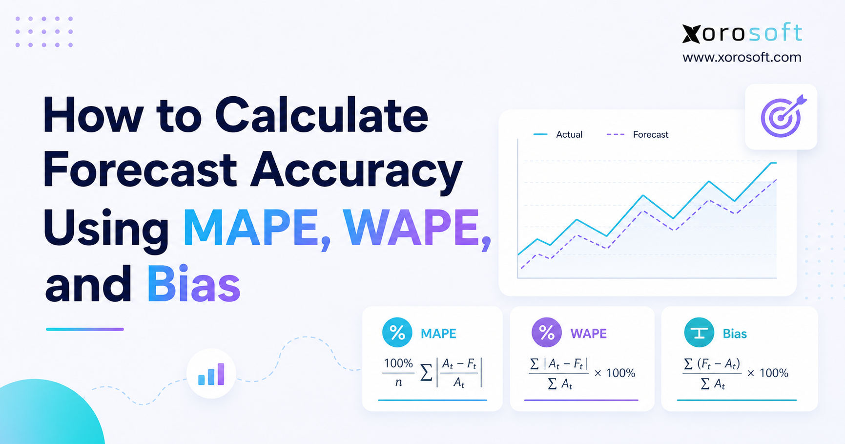
MAPE = (1 ÷ n) × Σ |(Actual − Forecast) ÷ Actual| × 100
MAPE remains popular because percentages give operations, finance, purchasing, and management teams an intuitive way to discuss forecasting performance.
Instead of telling an executive that average absolute error was 137 units, a planner can say that the forecast missed actual demand by an average of 9%. That percentage often makes cross-functional conversations easier, especially when the business sells products with different unit volumes.
3.2 MAPE Forecast Accuracy Example
Assume a company forecast 90 units of a product, while customers actually demanded 100 units.
The absolute error is:
|100 − 90| = 10
The absolute percentage error is:
10 ÷ 100 × 100 = 10%
Now assume five periods produce absolute percentage errors of 10%, 8%, 12%, 6%, and 9%.
The MAPE calculation becomes:
MAPE = (10 + 8 + 12 + 6 + 9) ÷ 5
MAPE = 9%
The forecasts missed actual demand by an average absolute percentage of 9% across those five periods.
MAPE does not tell you whether the business mostly forecast too high or too low. It only measures the average magnitude of the percentage errors.
3.3 Why MAPE Can Distort Forecast Accuracy for Low-Volume SKUs
MAPE has a major weakness: the formula divides each error by actual demand.
If actual demand equals zero, MAPE becomes undefined because the calculation requires division by zero.
Near-zero demand creates another problem.
Imagine one SKU sells 1,000 units and another sells only two. Missing the first SKU by 100 units produces a 10% percentage error. Missing the second SKU by three units produces a 150% percentage error.
If planners simply average those percentages, the tiny-volume item can exert disproportionate influence over the result.
This problem appears frequently in businesses that manage intermittent demand, spare parts, fashion variants, long-tail ecommerce catalogs, specialty wholesale products, or slow-moving industrial items.
MAPE still has value, but planners should understand what the metric rewards and penalizes before using it as a primary KPI.
3.4 Should You Convert MAPE Into a Forecast Accuracy Percentage?
Some businesses calculate:
Forecast Accuracy % = 100% − MAPE
If MAPE equals 9%, this approach produces a forecast accuracy percentage of 91%.
The calculation looks intuitive, but it can create confusion. MAPE can exceed 100%, especially when actual demand remains small relative to the forecasting error. In those cases, subtracting MAPE from 100 can produce a negative “accuracy” percentage.
For reporting, it is often clearer to present the error metric directly:
MAPE = 9%
rather than converting it into a potentially misleading accuracy score.
4. How to Calculate Forecast Accuracy With WAPE
4.1 WAPE Forecast Accuracy Formula
WAPE stands for Weighted Absolute Percentage Error.
The formula is:
WAPE = Σ|Actual − Forecast| ÷ Σ|Actual| × 100
Instead of calculating a separate percentage for every observation and averaging those percentages, WAPE combines the absolute errors and compares them with total actual demand.
That difference gives higher-volume products or periods more influence over the final metric.
4.2 WAPE Forecast Accuracy Example
Suppose actual demand totals 1,000 units across several periods.
The company’s total absolute forecast error equals 120 units.
The calculation becomes:
WAPE = 120 ÷ 1,000 × 100
WAPE = 12%
The business produced absolute forecast errors equal to 12% of total actual volume.
For many inventory teams, that interpretation makes WAPE useful when reviewing demand across a portfolio with very different SKU volumes.
4.3 MAPE vs. WAPE for Inventory Forecast Accuracy
Consider two products.
Product A sells 10,000 units.
Product B sells 20 units.
MAPE first calculates the percentage error for each observation and then averages those percentages. A large relative error on Product B can therefore materially affect the final score even though Product B represents a tiny portion of the company’s total demand.
WAPE evaluates the absolute errors against total actual volume, so Product A naturally carries more weight.
This often aligns better with inventory planning when high-volume products drive most purchasing, storage, fulfillment, and working-capital requirements.
However, WAPE does not automatically make SKU-level problems irrelevant. A low-volume SKU may still be strategically important, highly profitable, difficult to replenish, or essential to a major customer.
4.4 Why WAPE Is Not Always the Best Forecast Accuracy Metric
WAPE solves some problems but introduces limitations of its own.
If total actual demand equals zero, WAPE becomes undefined.
WAPE can also hide individual SKU problems because strong performance on high-volume products may overwhelm poor forecasting on smaller items.
Trending and highly seasonal demand can create additional interpretation challenges when teams compare WAPE across periods with substantially different demand levels.
The practical objective is not to decide whether MAPE or WAPE is universally superior. Instead, select the metric that reflects the planning problem, and retain enough detail to investigate exceptions.
5. How Forecast Bias Complements Forecast Accuracy Metrics
5.1 Forecast Bias Formula for Measuring Forecast Direction
MAPE and WAPE remove error direction because both rely on absolute error.
Forecast bias keeps the sign of the error.
Using the convention in this article:
Bias % = Σ(Forecast − Actual) ÷ Σ|Actual| × 100
Under this convention, a positive bias indicates over-forecasting, while a negative bias signals under-forecasting. When bias reaches zero, the forecast has no net directional error across the observations being measured.
5.2 Positive Forecast Bias and Overstock Risk
Imagine a company that repeatedly forecasts 10% more demand than customers actually generate.
The business may respond by purchasing more products, materials, or capacity than necessary.
Over time, persistent positive bias can contribute to excess inventory, slower inventory turnover, increased storage requirements, aged stock, markdown exposure, and unnecessary working-capital consumption.
Bias does not prove that forecasting caused every excess-inventory problem, but it gives planners a useful signal to investigate.
5.3 Negative Forecast Bias and Stockout Risk
Persistent negative bias indicates that actual demand regularly exceeds the forecast under the convention used here.
That pattern can contribute to insufficient purchase orders, material shortages, stockouts, lower fill rates, emergency supplier orders, and production pressure.
The correct response is not automatically to increase every forecast. Teams should determine whether the bias comes from seasonality, promotions, new customers, stockout distortion, model assumptions, manual overrides, or changes in demand.
5.4 Always Document Your Forecast Bias Sign Convention
Some businesses calculate:
Actual − Forecast
instead of:
Forecast − Actual
That reverses the interpretation of positive and negative bias.
Neither convention is inherently incorrect. Confusion begins when dashboards, analysts, spreadsheets, or software platforms use different conventions without explaining them.
Every forecasting report should clearly define the formula it uses.
6. MAPE vs. WAPE vs. Bias: A Complete Forecast Accuracy Example
6.1 Forecast Accuracy Dataset
Consider six periods of demand:
| Period | Actual | Forecast | Forecast Error | Absolute Error | Absolute % Error |
|---|---|---|---|---|---|
| 1 | 100 | 110 | +10 | 10 | 10.00% |
| 2 | 120 | 115 | -5 | 5 | 4.17% |
| 3 | 80 | 90 | +10 | 10 | 12.50% |
| 4 | 150 | 135 | -15 | 15 | 10.00% |
| 5 | 90 | 100 | +10 | 10 | 11.11% |
| 6 | 160 | 150 | -10 | 10 | 6.25% |
| Total | 700 | 700 | 0 | 60 | — |
6.2 Calculating MAPE Forecast Accuracy
Add the six absolute percentage errors:
10.00 + 4.17 + 12.50 + 10.00 + 11.11 + 6.25 = 54.03
Divide by six:
MAPE ≈ 9.00%
The forecasts produced an average absolute percentage error of approximately 9%.
6.3 Calculating WAPE Forecast Accuracy
Total absolute error equals 60 units.
Total actual demand equals 700 units.
WAPE = 60 ÷ 700 × 100
WAPE ≈ 8.57%
Total absolute forecast error therefore represents approximately 8.57% of actual demand.
6.4 Calculating Forecast Bias
Total forecast demand equals 700 units, and total actual demand also equals 700 units.
Bias = (700 − 700) ÷ 700 × 100
Bias = 0%
6.5 What These Forecast Accuracy Metrics Actually Tell You
| Metric | Result | Interpretation |
| MAPE | 9.00% | Average relative percentage error is about 9% |
| WAPE | 8.57% | Total absolute error equals 8.57% of actual volume |
| Bias | 0% | Over- and under-forecast errors cancel overall |
The bias result deserves attention.
A planner who sees 0% bias might assume the forecast performed perfectly. It did not. Across the six periods, the forecast accumulated 60 units of absolute error.
Bias only says the errors balanced directionally.
A practical forecasting scorecard should therefore combine an error-magnitude metric with a directional metric.
7. Choosing the Right Forecast Accuracy Metric for Demand Planning
7.1 Use MAPE Forecast Accuracy When Percentage Interpretation Matters
MAPE works well when actual values remain comfortably above zero and planners want an intuitive average percentage error.
It can help teams compare relative forecasting performance across products with different unit scales, provided low-volume and zero-demand observations do not distort the analysis.
7.2 Use WAPE Forecast Accuracy When Demand Volumes Differ Significantly
WAPE often makes sense when a company wants a portfolio-level metric that reflects actual demand volume.
If one product sells 50,000 units and another sells 50, weighting the higher-volume item more heavily may better reflect the operational significance of forecast error.
7.3 Use Forecast Bias Alongside MAPE or WAPE
Bias answers a different question.
MAPE and WAPE tell you how large forecast errors were, while bias shows whether those errors systematically pointed in one direction.
A business with acceptable WAPE but persistent positive bias may still carry too much inventory. Conversely, a company with acceptable MAPE but persistent negative bias may continue experiencing shortages.
7.4 Consider Other Forecast Accuracy Metrics When Demand Patterns Require Them
MAPE, WAPE, and bias do not cover every forecasting situation.
Other measures include Mean Absolute Error, Root Mean Squared Error, Mean Absolute Scaled Error, and Root Mean Squared Scaled Error.
Intermittent demand, new products, irregular order patterns, highly seasonal products, and rapidly trending demand may require different metrics or a combination of statistical and operational KPIs.
8. How to Measure Forecast Accuracy Across SKUs, Warehouses, and Channels
8.1 SKU-Level Forecast Accuracy Reveals Problems Aggregates Can Hide
Executive dashboards often show company-wide forecast performance.
Buyers, however, purchase specific SKUs.
A business can report good aggregate WAPE while repeatedly missing demand for critical products.
Consider apparel. A style may perform close to forecast at the total level while individual sizes and colors remain badly imbalanced. The business may hold plenty of inventory overall but still stock out of medium black units while carrying excessive inventory in less popular variants.
SKU-level forecast accuracy helps identify those exceptions.
8.2 Category-Level Demand Forecast Accuracy Supports Buying Decisions
Individual SKU data can become noisy, especially across large catalogs.
Category-level forecasting gives buyers another layer of context. If an entire product family consistently shows negative bias, the issue may involve category growth rather than an isolated SKU problem.
Companies should therefore create a measurement hierarchy that lets planners move from company to category to SKU.
8.3 How Warehouse Forecast Accuracy Improves Multi-Location Planning
Total demand can look accurate while inventory sits in the wrong location.
Suppose a company correctly forecasts 5,000 total units but overestimates East Coast demand by 500 units and underestimates West Coast demand by the same amount.
The company-level forecast looks excellent. Operationally, teams may still pay for stock transfers, longer shipping distances, split orders, or poor regional availability.
Businesses with multiple distribution centers should measure demand where replenishment and allocation decisions occur.
For operations that need tighter control over inventory by location, XoroWMS provides a warehouse-management layer for inventory-driven businesses that need more structured warehouse execution and multi-location visibility.
8.4 How to Measure Demand Forecast Accuracy by Sales Channel
Shopify, Amazon, wholesale, EDI, retail stores, and direct B2B channels can produce very different demand patterns.
A major wholesale order may create a large monthly spike without changing ecommerce demand. A Shopify promotion can affect direct-to-consumer sales while leaving wholesale demand largely unchanged.
Channel-level forecast accuracy helps teams separate those behaviors before combining demand into an overall inventory plan.
For Shopify merchants evaluating operational integrations, the Xorosoft ERP app on the Shopify App Store provides another reference point for connecting Shopify order and inventory workflows with broader ERP operations.
8.5 Forecast Horizon Should Be Part of Every Forecast Accuracy Review
A seven-day forecast and a six-month forecast answer different planning questions.
Short-term forecasts typically incorporate more recent information. Long-term forecasts must account for greater uncertainty around promotions, supplier conditions, seasonality, new customers, product launches, market shifts, and other changes.
Measure each horizon against a realistic business decision.
If purchasing needs a 120-day supplier lead time, evaluate the 120-day forecast rather than only the final short-term forecast.
9. How to Calculate Forecast Accuracy in Excel or Google Sheets
9.1 Spreadsheet Structure for MAPE, WAPE, and Bias
A simple spreadsheet can calculate all three metrics effectively when the dataset remains manageable.
Assume:
- Column B contains actual demand.
- Column C contains forecast demand.
- Column D contains forecast error.
- Column E contains absolute error.
- Column F contains absolute percentage error.
The formulas below give teams a practical starting point.
9.2 Excel Formula for Forecast Error
Enter:
=C2-B2
A positive value indicates over-forecasting under the convention used in this article.
9.3 Excel Formula for Absolute Forecast Error
Enter:
=ABS(C2-B2)
This removes direction and preserves only the size of the miss.
9.4 Excel Formula for MAPE Forecast Accuracy
For the individual absolute percentage error, use:
=IFERROR(ABS((B2-C2)/B2),"")
Then average the valid percentages:
=AVERAGE(F2:F100)
The IFERROR component prevents Excel from displaying a division error when actual demand equals zero, but teams should still investigate those zero-demand observations rather than simply ignoring their business meaning.
9.5 Excel Formula for WAPE Forecast Accuracy
Use:
=SUM(E2:E100)/SUM(B2:B100)
Format the result as a percentage.
9.6 Excel Formula for Forecast Bias
Use:
=(SUM(C2:C100)-SUM(B2:B100))/SUM(B2:B100)
For normal non-negative unit-demand data, this calculates bias using the Forecast − Actual convention described earlier.
Spreadsheets make the mathematics straightforward. At scale, the bigger challenge often becomes maintaining trustworthy actuals, forecast versions, SKU hierarchies, channel assignments, and warehouse data.
10. Forecast Accuracy Mistakes That Lead to Poor Inventory Decisions
10.1 Treating Recorded Sales as True Demand During Stockouts
Sales and demand are not always the same.
Suppose a product sells 800 units and then runs out of stock halfway through the month. Recorded sales equal 800 units, but customers may have purchased 1,100 units if inventory had remained available.
If the original forecast was 1,000 units, comparing that forecast with 800 recorded sales could make the company think it over-forecast demand.
In reality, the stockout may have constrained sales.
Teams should flag stockout periods and interpret historical actuals carefully.
10.2 Using the Same Forecast Accuracy Target for Every Product
A mature replenishment SKU with stable weekly sales does not behave like a new fashion collection.
Neither behaves like a low-volume replacement part.
Demand predictability changes by product lifecycle, volume, seasonality, lead time, promotion intensity, customer concentration, and other factors.
Forecast performance targets should therefore reflect product segments rather than one arbitrary company-wide threshold.
10.3 Ignoring Forecast Bias Because MAPE Looks Good
A planner can produce a reasonably low MAPE while still consistently forecasting in one direction.
Persistent over-forecasting may quietly build inventory, while persistent under-forecasting may repeatedly pressure service levels.
Review accuracy and bias together.
10.4 Averaging Forecast Accuracy at the Wrong Level
Simple averages can create misleading results when products vary significantly in demand volume.
If low-volume SKUs generate extreme percentage errors, company-wide MAPE can become difficult to interpret.
WAPE may offer a more useful volume-weighted view, but teams should still retain SKU-level visibility.
10.5 Ignoring New Products and Discontinued Items
New products lack enough history for conventional statistical forecasting.
Discontinued products create the opposite issue: historical demand may remain strong even though the company intentionally plans to stop replenishing them.
Teams should separate lifecycle decisions from model performance instead of treating every forecast error as a forecasting failure.
10.6 Comparing Different Forecast Horizons
A forecast made one week before demand occurs should not be compared directly with a forecast created six months earlier as though both represent the same planning challenge.
Standardize the horizon used for evaluation.
For purchasing teams, the most relevant horizon often relates to supplier lead time. Manufacturing teams may need a different window based on materials and production planning.
11. How to Improve Forecast Accuracy Without Chasing a Perfect Percentage
11.1 Improve Demand Data Before Replacing the Forecasting Model
When forecast accuracy deteriorates, teams often blame the algorithm first.
Data quality frequently deserves attention earlier.
Duplicate transactions, incorrect SKU mappings, missing sales, returns, inventory adjustments, unrecorded stockouts, one-time customer orders, and channel synchronization issues can distort the history used for forecasting.
A more sophisticated model cannot compensate for unreliable inputs indefinitely.
11.2 Segment Products by Demand Behavior
Fast-moving items, seasonal products, intermittent SKUs, new launches, and declining products should not automatically share the same forecasting logic.
Segmentation lets planners apply different methods, review thresholds, and exception rules based on demand behavior.
A high-volume replenishment item may justify a tight WAPE target. A new collection may require more judgment because the business has limited historical evidence.
11.3 Review Forecast Bias as a Process Signal
A single biased month may not mean much.
A persistent directional pattern does.
If one category remains positively biased quarter after quarter, investigate whether planners keep assuming growth that never materializes. If a warehouse consistently shows negative bias, examine whether regional demand has shifted faster than the planning process.
Bias can reveal behavior that absolute-error metrics hide.
11.4 Preserve Historical Forecast Versions
A forecast that changes every week needs version control.
Without historical versions, planners may accidentally compare actual demand with the latest prediction and overlook the forecast that originally drove the purchase order, supplier commitment, or production decision.
Preserving versions creates a more honest performance review.
11.5 Connect Forecast Accuracy to Business Outcomes
Do not stop at MAPE or WAPE.
Review whether forecasting errors correlate with stockouts, excess inventory, purchase-order changes, transfer activity, markdowns, service levels, working capital, or production changes.
That is where forecasting moves from analytics into operational improvement.
12. When Forecast Accuracy Requires Better ERP and Inventory Data
12.1 When Spreadsheet Forecast Accuracy Stops Scaling
Excel and Google Sheets can handle MAPE, WAPE, and bias calculations perfectly well.
For many smaller businesses, spreadsheets remain appropriate.
The problem begins when producing the inputs becomes harder than calculating the formulas.
A growing inventory business may need to combine data from Shopify, Amazon, wholesale orders, EDI, accounting software, warehouse applications, purchasing spreadsheets, manufacturing records, and multiple inventory locations.
At that point, analysts may spend more time reconciling information than evaluating demand.
The real question changes from:
“How do we calculate forecast accuracy?”
to:
“Do we trust the data feeding the forecast?”
12.2 Connected ERP Data Makes Forecast Accuracy More Actionable
An ERP system does not guarantee better forecasting.
No platform can remove uncertainty from customer demand.
A connected operational system can, however, reduce fragmentation between the forecast and the transactions that follow it.
XoroONE brings inventory, purchasing, accounting, warehouse management, manufacturing, forecasting, reporting, and ecommerce operations into a broader ERP environment for inventory-driven businesses.
That matters because a forecast should eventually influence action.
If demand increases, buyers may need to review purchase orders. When warehouse-level demand shifts, planners may need to change allocation. A manufacturing demand change can also require adjustments to materials and production requirements.
Forecasting becomes much more useful when those decisions share the same operational data.
12.3 ERP Forecasting Should Connect Purchasing, Inventory, and Accounting
Forecasting affects more than inventory quantities.
Purchasing decisions affect cash. Inventory affects financial reporting and working capital. Supplier commitments influence payment timing, while excess stock can create carrying costs and markdown risk.
XoroERP is relevant when a business needs its ERP, inventory, procurement, warehouse, manufacturing, and accounting processes to work within a more connected operating structure.
The broader principle applies regardless of software choice: forecasting should connect with execution.
A demand plan that never reaches purchasing or production remains only a prediction.
12.4 Compare ERP Platforms Against Operational Requirements
Businesses that outgrow disconnected tools often evaluate platforms such as NetSuite, Acumatica, Business Central, Cin7, Sage, Fishbowl, Brightpearl, or other ERP and inventory systems.
The right comparison should include inventory complexity, accounting requirements, warehouses, ecommerce channels, manufacturing, EDI, implementation requirements, reporting, integrations, and total operational fit.
For teams considering NetSuite specifically, Xorosoft provides a dedicated Xorosoft vs. NetSuite comparison that can serve as one reference point during a broader ERP evaluation.
13. Forecast Accuracy by Industry Requires Different Planning Context
13.1 Forecast Accuracy in Apparel and Fashion
Apparel businesses manage style, color, size, season, channel, and location combinations.
A category forecast can look accurate while individual size-color SKUs create stockouts and overstock at the same time.
Seasonality also raises the cost of mistakes because companies cannot always carry excess seasonal inventory indefinitely.
13.2 Forecast Accuracy in Furniture and Home Goods
Furniture introduces longer supplier lead times, high unit values, large storage requirements, and substantial freight considerations.
An over-forecast on a bulky product can create a very different working-capital and warehouse problem from the same percentage error on a low-cost accessory.
13.3 Forecast Accuracy in Sporting Goods
Sporting-goods demand can change with seasons, weather, events, geography, and product launches.
Teams should evaluate whether forecast errors come from the forecasting process or from event-driven demand that historical averages could not reasonably predict.
13.4 Forecast Accuracy in Food and Beverage
Food businesses must consider shelf life, batch controls, seasonality, and spoilage risk.
Over-forecasting may produce waste rather than simply slow-moving inventory, while under-forecasting can affect service levels during narrow selling windows.
13.5 Forecast Accuracy in Wholesale and Distribution
Wholesale businesses often face customer concentration.
One large customer’s order can materially change demand for a product or category.
Customer-level forecasts, EDI schedules, product-level demand, and aggregate inventory planning may therefore need separate accuracy reviews.
13.6 Forecast Accuracy in Manufacturing
Manufacturers need to translate finished-goods demand into components, raw materials, labor, and production requirements.
A forecast error on one finished product can propagate through a bill of materials and affect several purchasing decisions.
Businesses can review Xorosoft’s broader industry ERP solutions to see how inventory, wholesale, manufacturing, apparel, food, sporting goods, and other inventory-heavy operating models require different planning workflows.
14. Forecast Accuracy FAQs: MAPE, WAPE, Bias, and Demand Planning
14.1 What Is Forecast Accuracy?
Forecast accuracy measures how closely predicted values match actual demand. Businesses use metrics such as MAPE, WAPE, MAE, RMSE, and MASE to evaluate the size of forecast errors. Forecast bias adds directional context by showing whether forecasts systematically run above or below actual results.
14.2 How Do You Calculate Forecast Accuracy?
Match each forecast with the corresponding actual result and calculate the error. Then summarize those errors using an appropriate metric such as MAPE or WAPE. Calculate forecast bias separately to determine whether the forecasting process tends to over-forecast or under-forecast demand.
14.3 What Is the Forecast Accuracy Formula?
There is no single universal forecast accuracy formula. MAPE measures average absolute percentage error, while WAPE compares total absolute error with total actual demand. Bias measures directional error. The most useful formula depends on the products, demand pattern, forecast horizon, and business decision.
14.4 What Is MAPE in Forecasting?
MAPE means Mean Absolute Percentage Error. It calculates the average absolute percentage difference between forecast and actual demand. Companies often use MAPE because a percentage is easy to communicate, but zero and near-zero actual demand can make the metric difficult or impossible to interpret correctly.
14.5 How Do You Calculate MAPE?
Subtract forecast demand from actual demand, take the absolute value, divide by actual demand, and convert the result to a percentage. Repeat the calculation for each valid observation and average the individual absolute percentage errors.
14.6 What Does a MAPE of 10% Mean?
A MAPE of 10% means the average absolute percentage error across the observations equals 10%. It does not mean every forecast missed by exactly 10%, and it does not reveal whether the business generally forecast too high or too low.
14.7 What Is Considered a Good MAPE?
No universal MAPE threshold applies to every business. Product lifecycle, volatility, seasonality, forecast horizon, demand volume, data quality, and industry all affect forecast difficulty. Companies should create realistic benchmarks for comparable product segments instead of forcing one target across every SKU.
14.8 Can MAPE Exceed 100%?
Yes. MAPE can exceed 100% when forecast error becomes larger than the actual value. Small actual values make extreme percentage errors especially likely, which is one reason planners should use MAPE cautiously for low-volume and intermittent-demand products.
14.9 Why Does MAPE Fail When Actual Demand Is Zero?
MAPE divides absolute forecast error by actual demand. When actual demand equals zero, the calculation requires division by zero. That makes the individual percentage error undefined and limits MAPE’s usefulness for products with frequent zero-demand periods.
14.10 What Is WAPE in Forecasting?
WAPE means Weighted Absolute Percentage Error. It adds absolute forecast errors and divides that total by total actual demand. The approach naturally gives higher-volume products more influence over the aggregate result than lower-volume products.
14.11 How Do You Calculate WAPE?
Calculate the absolute error for every observation, add those errors, and divide the total by total actual demand. Multiply by 100 to express the result as a percentage. If absolute errors total 100 units against 1,000 actual units, WAPE equals 10%.
14.12 Is WAPE Better Than MAPE?
Not universally. WAPE can provide a more representative aggregate view when SKU volumes vary greatly, while MAPE offers intuitive percentage interpretation. Each metric has limitations, so planners should choose based on demand behavior and use additional measures when necessary.
14.13 What Is the Difference Between WAPE and WMAPE?
Terminology varies across software platforms and organizations. Some teams use WAPE and WMAPE for very similar formulas, while others apply explicit custom weights in WMAPE. Always review the underlying calculation rather than assuming identical metric names mean identical formulas.
14.14 What Is Forecast Bias?
Forecast bias measures whether forecasts systematically run above or below actual demand. Under the Forecast − Actual convention used in this article, positive bias indicates over-forecasting and negative bias indicates under-forecasting.
14.15 How Do You Calculate Forecast Bias?
Add forecast values, subtract total actual values, and divide the result by total absolute actual demand. Multiply by 100 to express bias as a percentage. Document the sign convention because some organizations reverse the subtraction order.
14.16 What Does Positive Forecast Bias Mean?
Under the convention used here, positive forecast bias means forecast demand exceeded actual demand overall. Persistent positive bias may indicate assumptions that contribute to excess purchasing, inventory accumulation, or unnecessary capacity commitments.
14.17 What Does Negative Forecast Bias Mean?
Negative forecast bias means actual demand exceeded the forecast overall under this article’s convention. Persistent negative bias can signal a tendency to under-plan inventory, purchasing, production, or capacity.
14.18 Is Forecast Bias the Same as Forecast Error?
No. Forecast error measures the difference between forecast and actual demand for an observation. Bias summarizes the net direction of those errors across multiple observations. Opposing errors can cancel, which means zero bias does not necessarily indicate high forecast accuracy.
14.19 Why Should Businesses Measure Bias With MAPE or WAPE?
MAPE and WAPE measure error magnitude but remove direction. Bias preserves direction but can hide offsetting errors. Tracking both gives planners a better view of how far forecasts miss and whether those misses consistently run high or low.
14.20 Which Forecast Accuracy Metric Works Best for Inventory Planning?
No single metric works best in every inventory environment. Many teams use MAPE or WAPE with forecast bias, then analyze results by SKU, warehouse, category, channel, and forecast horizon. Intermittent or highly volatile demand may require additional metrics.
14.21 Which Forecast Metric Works for Intermittent Demand?
MAPE often performs poorly when intermittent demand creates frequent zero or near-zero actual values. Teams may need absolute or scaled measures such as MAE or MASE, along with operational measures such as service levels and stockout frequency.
14.22 How Often Should Forecast Accuracy Be Measured?
Match the measurement cadence to the planning cadence. Weekly replenishment environments may review forecast performance weekly, while monthly planning teams may review monthly. Consistent forecast horizons matter more than simply increasing review frequency.
14.23 Should Forecast Accuracy Be Measured by SKU?
Yes, when the business makes purchasing, replenishment, allocation, or production decisions by SKU. Companies should also roll SKU results into category, warehouse, channel, and company-level views so planners can identify both individual exceptions and broader patterns.
14.24 How Do Stockouts Affect Demand Forecast Accuracy?
Stockouts can make recorded sales lower than true customer demand. If teams use those constrained sales as actual demand, a reasonable forecast may appear too high. Planners should flag stockout periods and account for lost-demand effects where possible.
14.25 How Does Forecast Accuracy Affect Safety Stock?
Forecast error contributes to uncertainty around future demand. When demand becomes less predictable, businesses may need additional protection through safety stock or other planning policies. Forecast accuracy should not determine safety stock by itself, but planners should consider forecast variability alongside lead time, service targets, and demand variability.
14.26 Can Forecast Accuracy Be Calculated in Excel?
Yes. Excel can calculate forecast error, MAPE, WAPE, bias, MAE, and many other metrics using standard formulas. Spreadsheets work particularly well when data volumes remain manageable and teams can maintain consistent forecast versions and reliable actual-demand data.
14.27 What Causes Poor Forecast Accuracy?
Common causes include unreliable historical data, stockouts, promotions, changing seasonality, new products, customer concentration, unexpected large orders, manual overrides, inconsistent forecast horizons, and forecasting methods that do not fit the product’s demand pattern.
14.28 How Can a Business Improve Forecast Accuracy?
Start with clean historical data, segment products by demand behavior, preserve forecast versions, measure bias, identify stockout periods, compare consistent forecast horizons, and review results at the SKU, category, warehouse, and channel levels. Model sophistication matters, but process and data quality often matter just as much.
14.29 Can ERP Software Improve Forecast Accuracy?
ERP software cannot guarantee better forecast accuracy. It can help by bringing sales, inventory, purchasing, warehouse, manufacturing, and accounting information into a more connected environment. Better access to consistent operational data can make forecasting analysis and the decisions that follow it easier to manage.
14.30 When Should a Business Move Beyond Spreadsheet Forecasting?
Consider moving beyond spreadsheets when data collection and reconciliation become harder than the forecasting calculations themselves. Multiple warehouses, thousands of SKUs, ecommerce channels, EDI, manufacturing, purchasing teams, and disconnected accounting or inventory systems commonly create that tipping point.
15. Conclusion: Use Forecast Accuracy to Drive Better Inventory Decisions
Forecast accuracy becomes valuable when it changes what the business does next.
MAPE helps teams understand average relative error, while WAPE provides a volume-weighted view of total absolute error. To complete the picture, forecast bias shows whether predictions systematically run above or below actual demand.
No single metric should operate in isolation.
Measure forecasts at the level where decisions occur. Review SKU, category, warehouse, channel, and forecast-horizon performance. Separate stockouts from true demand, preserve historical forecast versions, and segment products according to demand behavior.
Most importantly, connect forecast performance with inventory, purchasing, production, customer service, and working-capital outcomes.
A simple operation may accomplish all of this effectively in Excel or Google Sheets. As SKU counts, warehouses, sales channels, purchasing processes, manufacturing requirements, and financial workflows become more complex, the data infrastructure behind forecasting often matters as much as the forecasting model itself.
For businesses reaching that point, Xorosoft provides ERP, inventory, warehouse, purchasing, manufacturing, accounting, and ecommerce capabilities designed around inventory-driven operations.
The right next step is not to buy software simply because MAPE or WAPE looks weak. Identify where the planning process breaks down, determine which data and workflows remain disconnected, and evaluate whether a more integrated operating system would materially improve the decisions your team makes.
If your business is evaluating that transition, contact Xorosoft for a personalized discussion and demo.
Recent Posts
-
 Xorosoft vs NetSuite for Shopify B2B Operations in 2026
 -
 How to Manage Shopify B2B Payment Terms Without Breaking AR and Order Release
 -
 Supplier Performance Benchmarks 2026: Lead Time, Fill Rate, and Defects
 -
 Inventory Management for Target Plus Sellers Expanding Beyond Shopify
 -
 What Is an ERP Conference Room Pilot and Why Should Buyers Require One?